Clip your lidar file

Because most of these lidar files are ENORMOUS, we’re going to clip it to make it more manageable (and to zoom in on subsections if you’re into that). I added a growth variable because I wanted to play around with the size without having to do a lot of converting in my head.

#Clipping box in lat-lon
growth = .002

xmin1 = -122.671 - 2*growth
xmax1 =  -122.642 + 2*growth
ymin1 = 45.293-growth 
ymax1 = 45.306+growth

# make it a cropping box
castle_Crop_Lat <- rast(xmin=xmin1, xmax = xmax1, 
                        ymin = ymin1, ymax = ymax1)

Project Your Raster

Ok, don’t just project your big ol’ lidar image or you’ll be sitting here for a very long time. Instead, clip the raster first and then project your much smaller object. That means you need to take your nice tidy little crop box, project it to have the same coordinates as the bigger lidar image, and then use that to crop. Then project your cropped lidar file into something a bit more coherent than the default lidar projection.

# make your cropping box the right projection
castle_Crop_Box <- project(castle_Crop_Lat, crs(castle))

#now crop the castle lidar
castle_cropped <- crop(castle, castle_Crop_Box)


#project your cropped castle lidar back into 
#a reasonable projection
castle1 <- project(castle_cropped,"EPSG:4326")

If you stop here, your lidar will look kinda wonky becase the original projection was in a weird conic thing. So now you re-crop it to make it a square shape.

# make it back into a square shape 
castle2 <- crop(castle1, castle_Crop_Lat)

Create Underlying Layers

To make a red relief image you need to have a few different layers. The top layer will be the slope. The bottom layer will either be a digital elevation model (DEM) or a hillshade model (sparkly extra DEM).

You have the DEM. That’s what you got. It’s also called a DTM, to make your life maximally confusing.

But you don’t have a hillshade layer or a slope layer. So let’s make those. And since aspect is required to make a hillshade model, you’ll need to make that too. You can make those requirements using terrain() from terra. I am specifying terra here because inevitably when making maps I somehow have another R tab open where i load the raster library and as a result, suddenly the terrain function doesn’t work as expected.

castle.slope <-  terra::terrain(castle2, v= "slope", 
                                neighbors = 8, unit = "radians")
castle.asp <-  terra::terrain(castle2, v= "aspect", 
                              neighbors = 8, unit = "radians")

Now, use those to make the hillshade map in case you think it’s prettier.

castle.hill <- shade(slope=castle.slope, 
                     aspect=castle.asp, 
                     direction = 140)

Get Set Up For ggplot2

I like to mess around with this stuff in ggplot, which doesn’t like rasters the way I do. That means it’s easier to transform the rasters into data frames, using as.data.frame() from terra.

castle3 <- as.data.frame(castle2, xy = TRUE)
colnames(castle3) <- c("x", "y", "z")
castle.slope2 <- as.data.frame(castle.slope, xy = TRUE)
colnames(castle.slope2) <- c("x", "y", "z")
castle.hill2 <- as.data.frame(castle.hill, xy = TRUE)
colnames(castle.hill2) <- c("x", "y", "z")

Plot Base Layers

Now we are ready to plot! Remember these maps are made with two different types of plots - hillshade, and plain old vanilla DEM. Here we can make them and you can cross-compare them at your leisure.

hill.plot <- ggplot()+
  geom_raster(data = castle.hill2, aes(x=x, y=y, fill = z))+
  scale_fill_gradient2(low = "black", 
                       mid = "grey50", 
                       high = "grey92", 
                       midpoint=.8)

hill.plot + labs(title = "Hillshade Plot")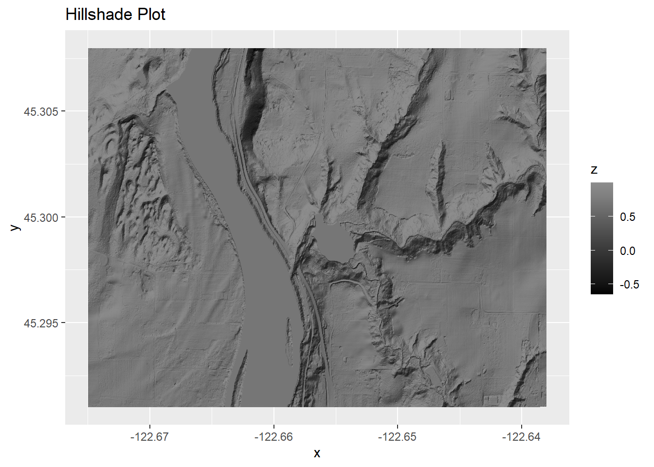

DEM.plot <- ggplot()+
  geom_raster(data = castle3, aes(x=x, y=y, fill = z))+
  scale_fill_gradient2(low = "black",
                       mid = "grey50", 
                       high = "grey92", 
                       midpoint=180)

DEM.plot +  labs(title = "DEM Plot, Meaghan's Favorite")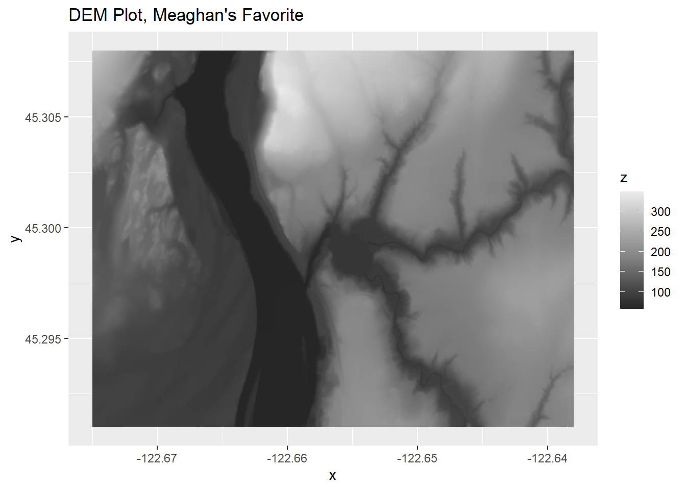

A big part of making these look nice is playing around with the gradient fill component and picking a nice midpoint that makes everything highlighted really well. You can do that by randomly entering numbers or be a bit more methodical by looking at a histogram and picking something slightly higher than the center.

hist(castle.hill2$z)
abline(v = .8, col = "red")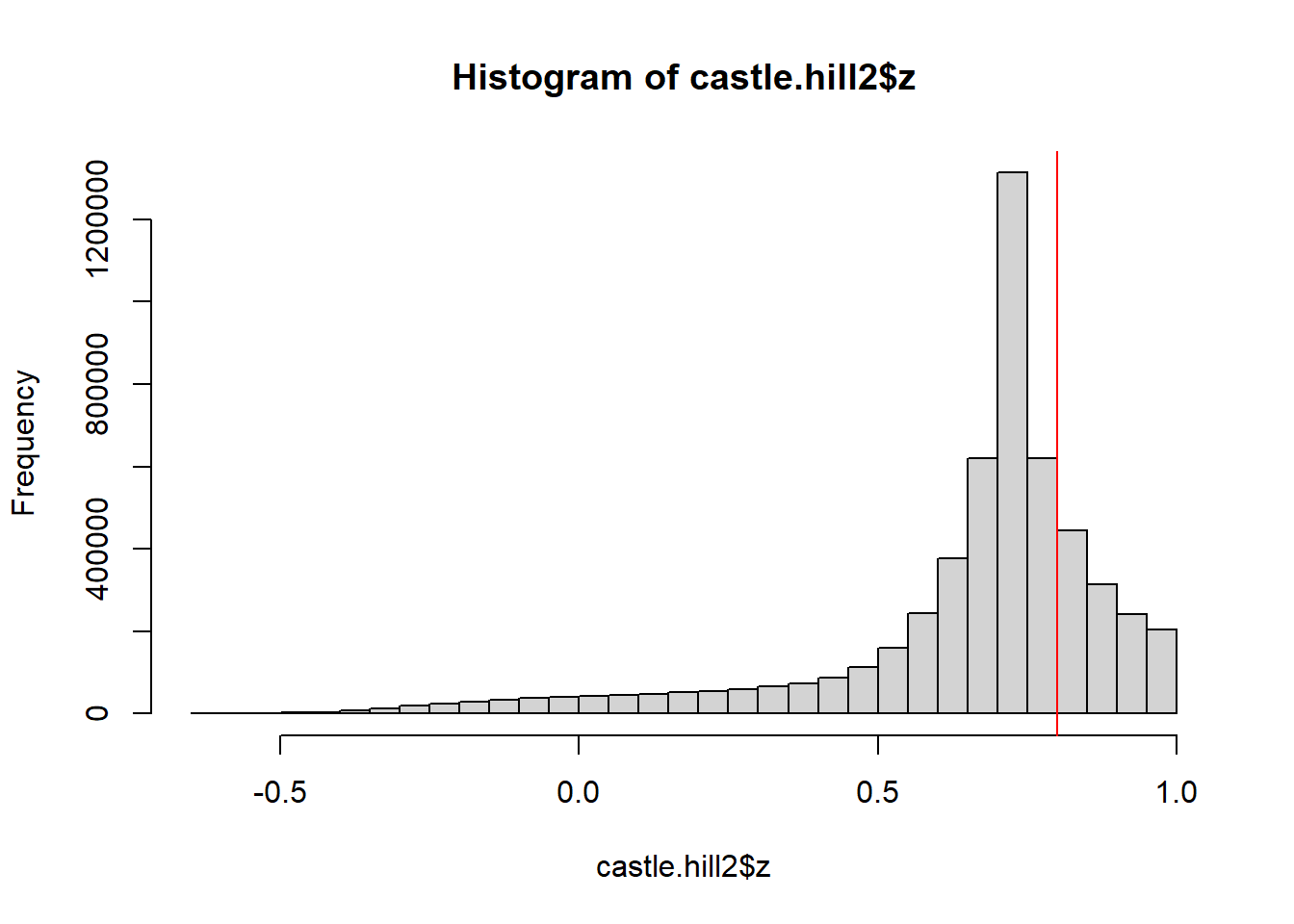

Plot the Slope Raster

Now, we add on a slope raster. Red is classic (hence red relief) but you can use other colors here! I’m using some changing transparency as well with the alpha() function, to make it so that steeper slopes are both darker and more opaque.

slope.plot <- DEM.plot +
  new_scale_fill()+
  geom_raster(data = castle.slope2, 
              aes(x=x, y=y, fill = z), alpha = .25)+
  scale_fill_gradient(low = alpha("pink", .0001), 
                      high = alpha("firebrick", .3))

slope.plot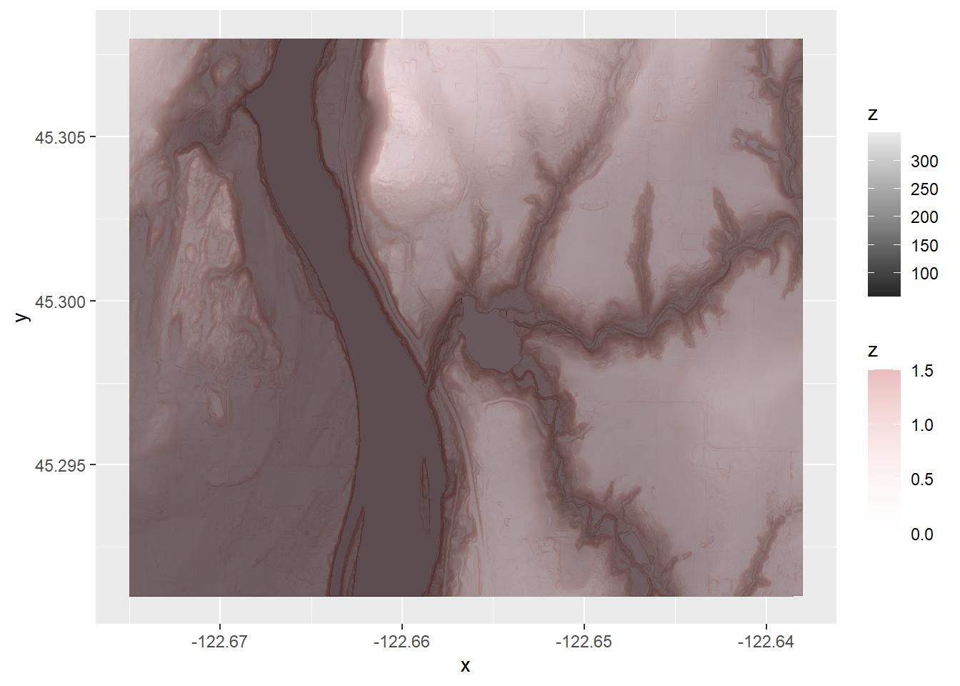

Prettify the Plot

Now, add in the things that make this prettier! That includes clipping the sides of the plot using the expand argument, adding a white border to avoid showing off how awkwardly you clipped it, etc. That last bit only matters when you print out the file btw, but I can assure you otherwise the white border your printer chooses will be a seriously mismatched rectangl.

And of course, this is where you turn off annoying lat/lon coordinates and legend items using theme_void(). Why? Because red relief maps are about vibes, not about specific reconstructions that require you to know what slope percentage exactly you’re looking at.

final.plot <- slope.plot +
  theme_void()+
  theme(legend.position = "none")+
  scale_x_continuous(limits = c(xmin1, xmax1), 
                     expand = c(0,0)) +
  scale_y_continuous(expand = c(0,0))+
  theme(plot.background = 
          element_rect(fill = "white", color = NA),
        plot.margin = 
          margin(15, 15, 15, 15),
        panel.border = 
          element_rect(color = "white", 
                       fill = NA, 
                       size = 4)) 

final.plot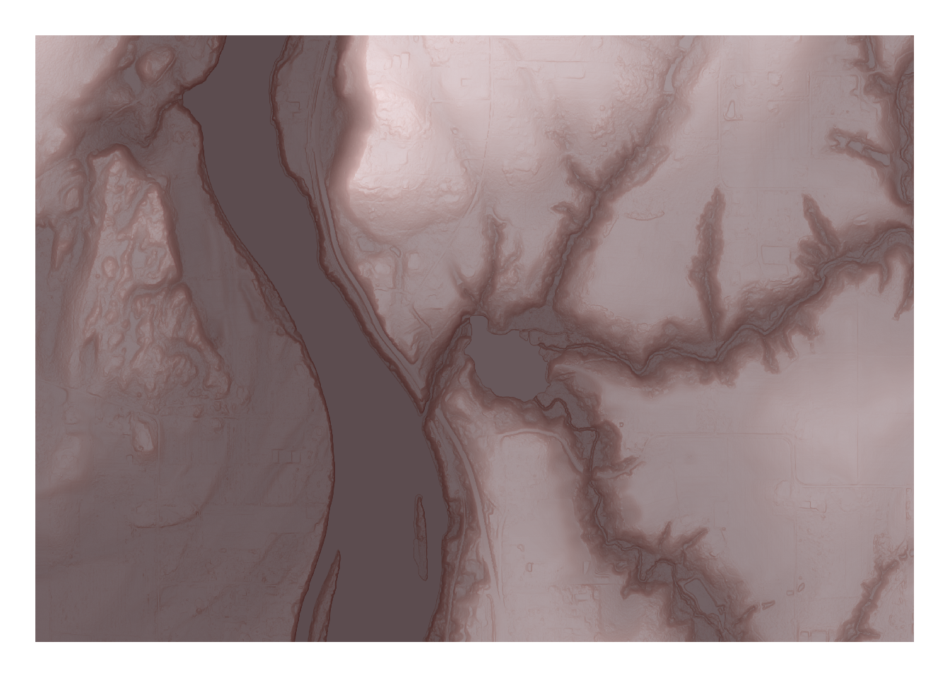

Export your plot

Finally, export it! Then you can print it, or make it a background. Or treasure it forever as an NFT or something, I don’t know. What I did was use these as an emergency Christmas present by making maps of people’s homes, which is only creepy if you don’t know those people very well or have been otherwise barred from their homes.

ggsave("castle 24x18.jpg", final.plot, dpi = 300, 
       width = 24, height = 18, units = "in")