You can skip to the bottom to just see the code.

Introduction

In a previous post I talked a lot about why ggplot2 has a terrible default color palette. In this post, I’ll show you how to use the colorBlindness package to quickly and easily determine if your particular color palette is equally garbage.

Packages

library(ggplot2) #graphics
library(ggplotify) # to convert to ggplot2
library(colorBlindness) #pretty self explanatory I'd say

Why colorBlindness

There are plenty of other packages that simulate colorblindness in R. colorBlindr, dichromat, and colorblindcheck come to mind. I’ve found that the only one that meets the following “make it easy” criteria is colorBlindness. Those criteria are:

is available on CRAN (colorBlindr is not)
can be run on plots, not lists of colors (colorblindcheck does not)
does not require editing your plots to run (dichromat technically replaces your colors)

Easy Mode: ggplot2 Graphics

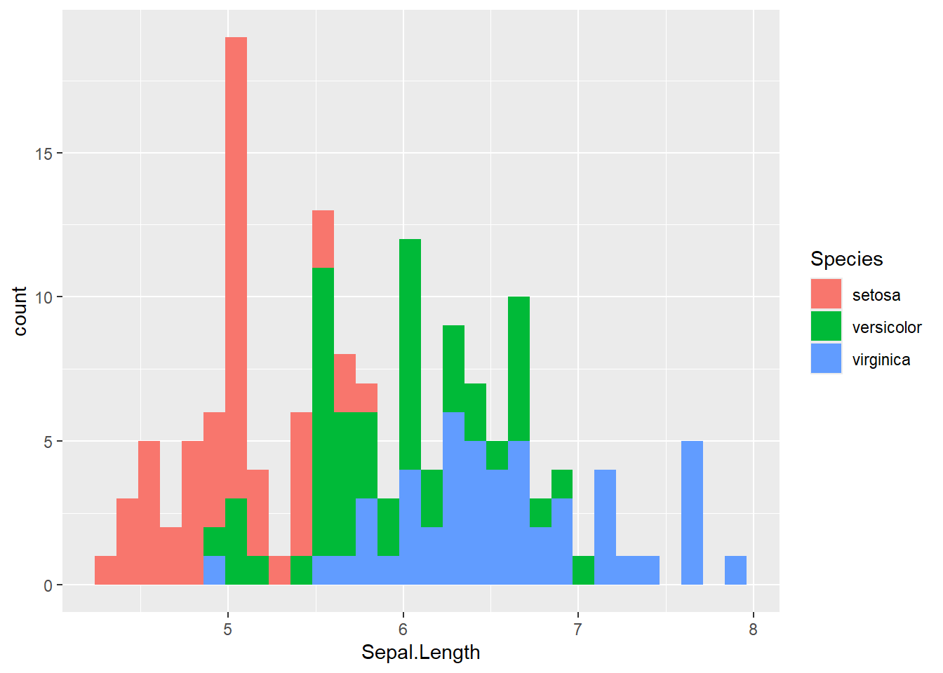
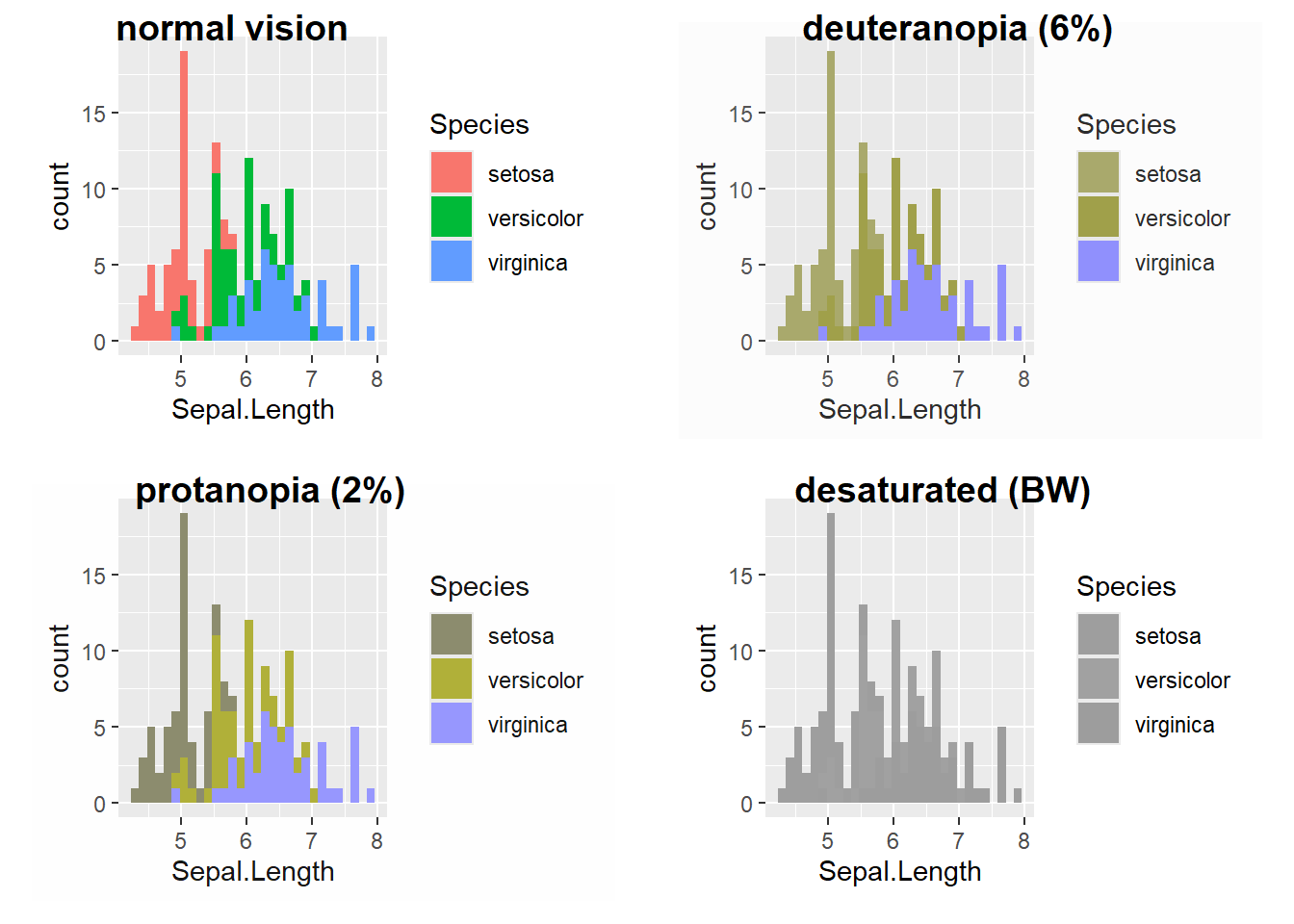
If you are using ggplot2 to make your graphics, checking your plots is insanely easy. You just run your ggplot code, then cvdPlot().

ggplot(data = iris, aes(x = Sepal.Length, fill = Species))+
  geom_histogram()

cvdPlot()

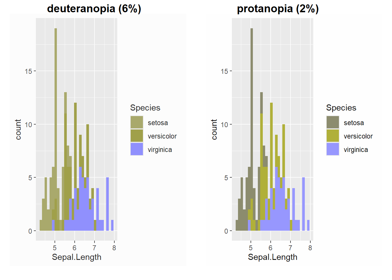
You can also save your ggplot and call it out, and specify exactly which variants of colorblindness you’d like to look at using the layout argument.

plot1 <- ggplot(data = iris, aes(x = Sepal.Length, fill = Species))+
  geom_histogram()

cvdPlot(plot1, layout=c("deuteranope", "protanope"))

Medium Mode: Base R plots

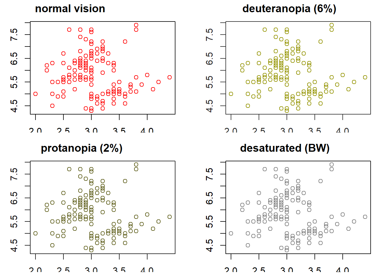
Base R plots need to be converted to ggplot items first. The easiest is to to use the as.ggplot() function from ggplotify. Add a tilda (~) in front of your plotting function to make this work.

plot2 <- as.ggplot(
     ~ plot(iris$Sepal.Length~iris$Sepal.Width, col="red")
                   )

cvdPlot(plot2)

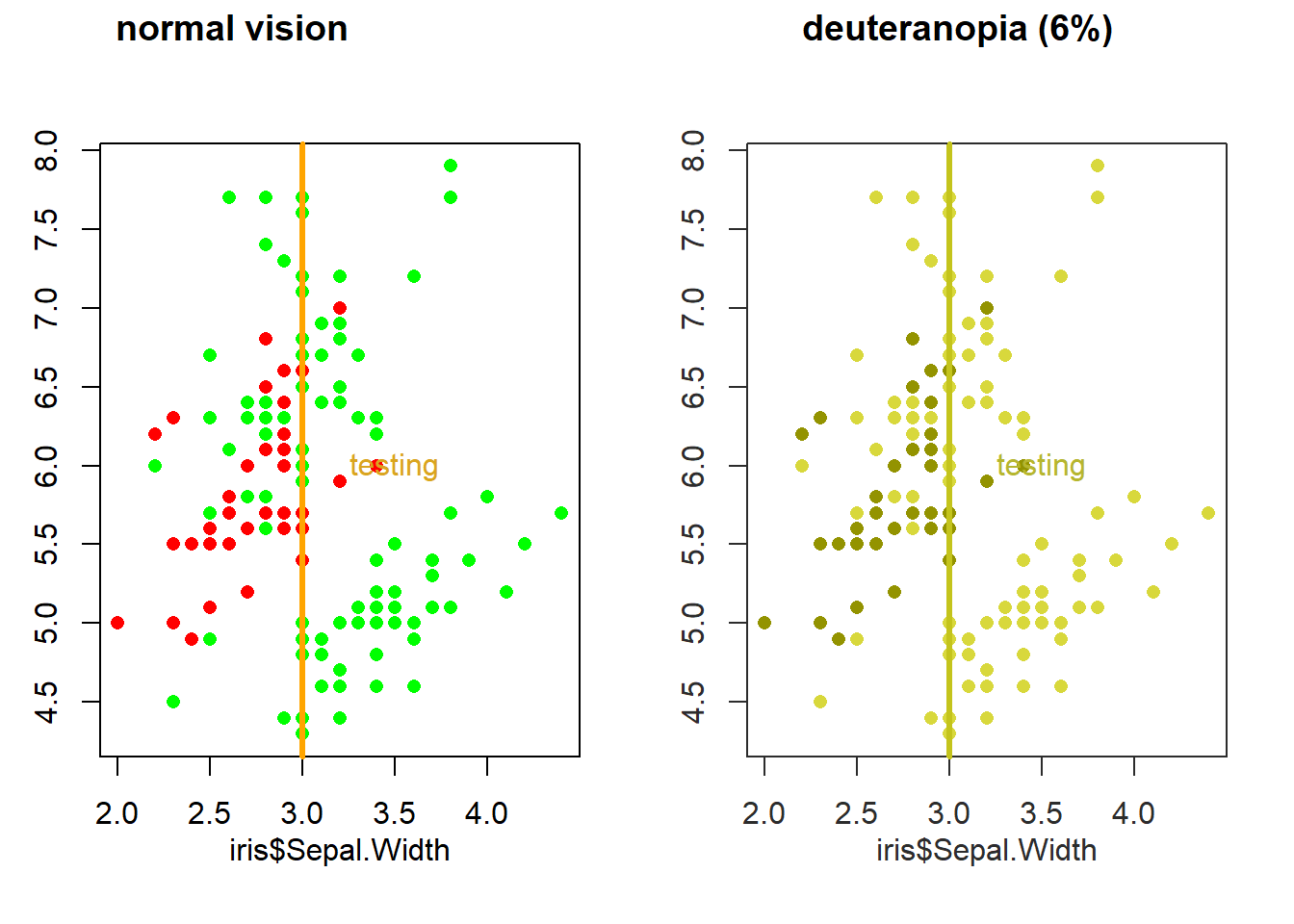
You can do this with more complex base R plots that use additional functions (or, you know, colors), even if they aren’t nested, by using a + to connect them. So for example, the following plot contains three non-nested functions (plot(), abline(), text()) but they work because the first function has a tilda (~) and the second and third have a plus (+).

plot3 <- as.ggplot(~ 
            plot(iris$Sepal.Length~iris$Sepal.Width,
                 col = ifelse(iris$Species == "versicolor", "red", "green"),
                 pch=16) +
            abline(v = 3, col = "orange", lwd = 3) +
            text(x = 3.5, y = 6, labels = "testing", col = "goldenrod")
                   )

cvdPlot(plot3, layout = c("origin", "deuteranope"))

Medium Hard Mode: Complicated Base R Plots

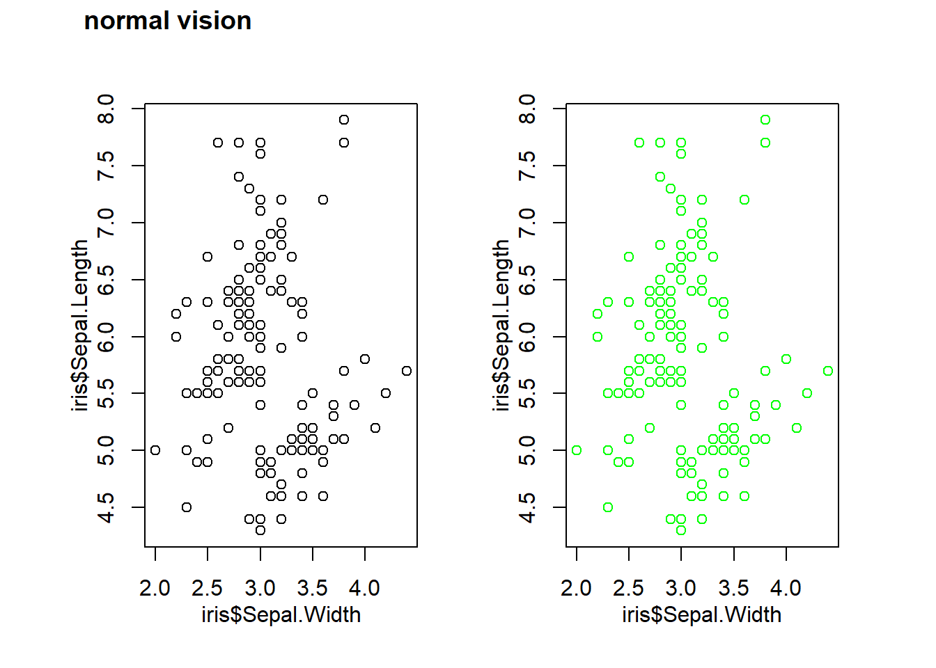
Unfortunately, base R plots are not storeable as objects in R the same way that ggplot items are. So if you have a tremendously complex base R plot, this method can be really annoying. And if the first function in your set of base R functions isn’t one of the default plotting functions, this can fail entirely. I did find that this was the case when trying to stack two plots together using something like par(), where the result was that only the second plot was captured in the ggplot object.

The easiest way I’ve found around this is to use a wrapper function that calls your plot. Put that in the as.ggplot() function with the tilda (~), and it works just fine.

testme <- function(){
  par(mfrow=c(1,2))
  plot(iris$Sepal.Length~iris$Sepal.Width)
  plot(iris$Sepal.Length~iris$Sepal.Width, col = "green")
}

plot5 <- as.ggplot(
           ~testme()
           )

cvdPlot(plot5, layout = "origin")

Possibly Impossible Mode: Raster Objects

The biggest flaw in colorBlindness in my opinion is that it is entirely designed to work on vector graphics, not raster. So if you are using external graphics or trying to make maps with things like lidar data, you run into issues. This will also crop up if you are using certain formats of images in your ggplot objects, like png files or logos.

I have played around with a lot of different possible solutions to this. I did not at any point find an ’easy’ method. If I do, I will come back and update this!

References and Further Reading

Hannah Weller. 2005. “Using the dichromat package to check if your plot is colorblind-friendly.”

Jianhong Ou. 2021. “colorBlindness: Safe Color Set for Color Blindness.”

Guangchuang Yu. 2025. “Convert plot to grob and ggplot object.”

The Code

Wanted just the code with no interruptions? K. Here you go.

library(ggplot2) #graphics
library(ggplotify) # to convert to ggplot2
library(colorBlindness) #pretty self explanatory I'd say

ggplot(data = iris, aes(x = Sepal.Length, fill = Species))+
  geom_histogram()

cvdPlot()

plot1 <- ggplot(data = iris, aes(x = Sepal.Length, fill = Species))+
  geom_histogram()

cvdPlot(plot1, layout=c("deuteranope", "protanope"))

plot2 <- as.ggplot(
     ~ plot(iris$Sepal.Length~iris$Sepal.Width, col="red")
                   )

cvdPlot(plot2)

plot3 <- as.ggplot(~ 
            plot(iris$Sepal.Length~iris$Sepal.Width,
                 col = ifelse(iris$Species == "versicolor", "red", "green"),
                 pch=16) +
            abline(v = 3, col = "orange", lwd = 3) +
            text(x = 3.5, y = 6, labels = "testing", col = "goldenrod")
                   )

cvdPlot(plot3, layout = c("origin", "deuteranope"))

testme <- function(){
  par(mfrow=c(1,2))
  plot(iris$Sepal.Length~iris$Sepal.Width)
  plot(iris$Sepal.Length~iris$Sepal.Width, col = "green")
}

plot5 <- as.ggplot(
           ~testme()
           )

cvdPlot(plot5, layout = "origin")

Is your plot colorblind friendly?